Bayesian Inference, Part 2: Fitting (Generalised) Linear Models

Preface

In the last post of this series, we looked at the basics of Bayesian model fitting both from an analytical and from a numerical perspective. In particular, we have fitted probability distributions to sets of measured values. In this post, we will look at another typical application of Bayesian inference: We will fit some of the "classical" statistical models used to describe the relationship between different variables.

In particular, we will first fit two of the most well-known linear models, the simple linear regression, and the ANOVA (analysis of variance) "the Bayesian way". Doing so, we will learn about the Python library "Bambi", which makes fitting models like this extremely easy. This approach extends easily to more complicated linear models such as the ANCOVA (analysis of covariance), or multiple linear regression. Finally, we will also look at one example of generalised linear models (the logistic regression); and we will use this specific example to also do some hypothesis testing on the model results.

Simple Linear Regression

We start with the arguably most famous statistical model -- the simple linear regression. Given a set of points in 2d space, we want to fit a linear function of the form

\(y = a + bx\); where \(a, b \in \mathbb{R}\).

Generating some data

Let's first generate some data to work with. We do so as follows:

This gives us the following dataset:

Fitting the model with PyMC3

Fitting a linear regression model to this dataset with PyMC3 is easy to do, although we will learn about another library that makes it even easier in a minute. For now, we fit the model using only PcMC3, because in this way we see more of what is going on "under the hood," which will give rise so some interesting observations. We do:

    from pymc3 import Model, Normal, Uniform, sample

    with Model() as model:  
        # Define priors
        # We need a function intercept, ... 
        intercept = Normal("intercept", 0, sigma=20)
        # ... a function slope, ...
        slope = Normal("slope", 0, sigma=20)
        # ... and the standard deviation of the residuals
        sigma = Uniform("sigma", 0, 10)
        
        # Define likelihood
        likelihood = Normal("y", mu=intercept + slope * x, sigma=sigma, observed=y)
        
        # Inference
        # draw posterior samples using NUTS sampling
        samples = sample(1000, return_inferencedata=True)
    

We can observe some interesting things here. First, note that we do not only need to fit our two parameters \(a, b\), but also a third one named sigma (\(\sigma\)). This variable \(\sigma\) corresponds to the standard deviation of the residuals, i.e. the deviations of the data points from the fitted linear models. We need to learn this variable, because the model structure of a linear regression (see the line starting with "likelihood = ") is actually a normal distribution of residuals around the line we fit. This means, when we are fitting a simple linear regression, we are actually learning a normal distribution "under the hood" -- or rather one normal distribution around every individual observed \(y\) value, all of which are sharing the same standard deviation \(\sigma\).

This is also the reason why we always need to make sure that our residuals are normally distributed with a constant standard deviation, when we are fitting a normal distribution the "classical" frequentist way (e.g. by using the lm() command in R).

An easier way of fitting the model -- using Bambi

Admittedly, specifying a simple model like a linear regression in this very detailled way every time may become a bit annoying and may lead to lots of boilerplate code. For this reason, Capretto et. al have written the Python library "Bambi", which builds upon PyMC3 and provides a very easy way of fitting many of the classical models used in biomedical research and the social sciences using the "tilde syntax" known from the R language. The documentation of the library is very comprehensive and definitely worth checking out.

Using this library, the whole procedure simplifies to:

    import bambi as bmb
    
    model = bmb.Model("y ~ x", data)
    samples = model.fit(draws=1000)
    

The attentive reader will probably have noted that we do not have specified any prior distributions here. This is because bambi is written to select some priors automatically which are as uninformative as possible. Of course, if we have prior knowledge available, or if we simply want to check whether our results are invariant to changes in priors, we need to manually change them -- for details on this refer to the documentation.

Let's inspect the results by using

    from arviz import plot_posterior
    ax = plot_posterior(samples2, figsize=(15,5), grid=(1,3), textsize=15);
    

We get:

To inspect the model parameters, we can use az.summary(samples), which gives us the following printout:

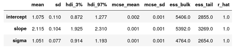
Looking great! As mentioned in the previous post of the series, we now need to do some sanity checks (which we omit here for the sake of brevity): we should check whether our model reproduces the input data accurately, we should make sure that our results are invariant to changes in our prior assumptions, and we might also want to look at the model traces (by using az.plot_trance(samples2, compcat=False)) to check whether the numerics have converged nicely.

ANOVA using Bambi

With the Bambi library, it becomes extremely easy to fit other well-known models such as the ANOVA, the ANCOVA with or without interaction term, multiple linear regression, etc. by simply changing the formula in the library call. We'll thus only provide one more example here, without going into any more detail.

ANOVA and all kinds of other linear models

We again generate some data first. We assume three groups with different means, around which our data is distributed normally with a constant standard deviation.

    # Parameters
    n = 100
    ybar1 = 1
    ybar2 = 5
    ybar3 = 10
    sigma = 0.5

    # Generate data
    np.random.seed(0)
    y1 = np.random.normal(ybar1, sigma, n)
    y2 = np.random.normal(ybar2, sigma, n)
    y3 = np.random.normal(ybar3, sigma, n)

    # Dataframe for bambi library
    x = ["a" for _ in range(n)] + ["b" for _ in range(n)] + ["c" for _ in range(n)]
    y = list(y1) + list(y2) + list(y3))
    data = pd.DataFrame(dict(x=x, y=y))
    

And we are already all set-up to fit the model:

    model = bmb.Model("y ~ x", data)
    samples = model.fit(draws=1000)
    

The library automatically recognises that x is now a categorical instead of a continuous predictor, thus instead of a simple linear regression, an ANOVA is fitted. Plotting the results by using

    plot_posterior(samples, figsize=(12,10), grid=(2,2), textsize=15);
    

we get

Again, the results are absolutely spot-on. Our global intercept (which here corresponds to the mean of the first group "a") is indeed 1.0, and the means of groups "b" and "c" are 4 or 8.9 units above that intercept, respectively. The standard deviation of the noise term is estimated to be 0.5, which is exactly what we chose for our data generation.

All kinds of other linear models such as an ANCOVA with or without interaction term, or a multiple linear regression can easily be fitted as well using exactly the same approach -- for this reason, we will omit further examples of linear models here for the sake of brevity.

Generalised linear models

Finally, we'll also fit a generalised linear model, i.e. a linear model where the response variable first undergoes some transformation. This is especially useful if we are e.g. dealing with binary yes/no (0/1) data, or count data (which both tend to lead to non-normal distributions and would thus violate the normality assumption of linear models).

As an example, consider an experiment where plant seeds of different species have been exposed to different temperatures, and the fraction of germinated seeds has been measured. For instance, we might want to compare three different plant species, which we call "Species A", "Species B", "Species C", across different temperature conditions of 0, 1, 2, ..., 20 degree Celsius. This gives us \(3 \times 21 = 63 \) experimental groups. Per group we plant 100 seeds and count the number of germinated seeds after some amount of time has passed.

This approach fits the description of a Bernoulli trial, so a generalised linear model with a logit link function, also called a "logistic regression" is the model of our choice. To generate artificial data to work with, we thus want to simulate drawing from a Binomial distribution, where the probability of a success is a function of our predictors "temperature" and "species." Hence, for each of the three species, we first choose an intercept \(a\) as "baseline germinating possibility" and a slope \(b\) that encodes the influence of our predictor "temperature", as if we were generating data for a simple linear regression. However, the response variable we get this way does not always fall neatly into the interval \([0;1]\), thus we cannot use that as probabilities for our Binomial distributions to draw from. Hence, we first transform it to fall into that interval using the inverse logit function, and then we can simply do the sampling. In Python, this looks like this:

    # Seed for reproducibility
    np.random.seed(0)

    # Temperatures
    temp = np.array([i for i in range(21)])

    # Intercept and slope for three plant species
    a1 = -5
    b1 = .5
    a2 = -2
    b2 = .75
    a3 = 5
    b3 = -1

    # The linear responses z ...
    z1 = a1+b1*temp
    z2 = a2+b2*temp
    z3 = a3+b3*temp

    # ... are transformed to fall into [0; 1]
    pr1 = 1/(1+np.exp(-z1))
    pr2 = 1/(1+np.exp(-z2))
    pr3 = 1/(1+np.exp(-z3))

    # Only then we can use them as probability for binomial experiments
    y1 = np.random.binomial(50, pr1)
    y2 = np.random.binomial(50, pr2)
    y3 = np.random.binomial(50, pr3)
    

Plotting the germination frequencies over temperature for the three species, we get nice sigmoid curves just like we get in real-life when working with data from Bernoulli trials:

For fitting the model, we first need translate the data into "long form", where every seed is one single line. This can be easily done with a simple loop, and we omit this step here for the sake of brevity. Then, we can fit the model as follows:

    model = bmb.Model("germ ~ temp*species", family="bernoulli", data=data)
    samples = model.fit(draws=1000)
    

This yields the following posteriors:

Generally, these results look very nice, only the global intercept (which equals the intercept of plant species "A") has been overestimated a bit (-4.6 instead of -5). Still, its true value falls within the 94% HDI. This suboptimal result is likely the consequence of the fact that we are estimating 6 parameters in parallel here. A bigger sample size would likely lead to more accurate estimates.

Let us also use this example to do some hypothesis testing, using the posterior distributions we have just obtained. For this, we roughly follow this part of the excellent docs of the bambi library. Assume we want to examine whether the slopes of the different plants' responses in germination probability to different temperature regimes differ significantly. For this, we first need to extract the posterior distributions of the parameters from our fitted model.

The estimates for the differences in slope are stored in samples.posterior["temp:species"]. In particular, samples.posterior["temp:species"] has a shape of \(4 \times 1000 \times 2\) elements, where the first dimension corresponds to the four independent models (or "chains") we fitted. The second dimension corresponds to the 1000 estimates per fitted model we obtained. Finally, in the third dimension, two values are stored -- the estimated difference in slope between plant species B compared to A, and the difference in slope between species C and A, respectively (these are also the values we have plotted before in the middle and right-hand side panel of the lower row). These we need to compare with zero. Let's first extract them into separate variables:

    diff_ba = samples.posterior["temp:species"][:, :, 0]
    diff_ca = samples.posterior["temp:species"][:, :, 1]
    

Because these two variables still contain multi-dimensional objects (to be more precise, they're lists of four lists, where every one of these four sub-list represents the results from one of the four independent chains), we use a convenience function for plotting their distributions:

    az.plot_kde(diff_ba, label="Slope B - Slope A", plot_kwargs={"color": "C0"})
    az.plot_kde(diff_ca, label="Slope C - Slope A", plot_kwargs={"color": "C1"})
    

This yields the following plot:

To quantify this, we can calculate how many of the slope estimates (across the four independent model chains) are larger or smaller than zero, by doing:

    np.mean(diff_ba>0)
    np.mean(diff_ca<0)
    

In both cases, we get a results of 1.0 -- that means, all of our 4000 estimates were larger or smaller than zero, respectively. Thus, we can be pretty sure that slopes B and A, and C and A are indeed different from each other -- which we of course also already knew for a fact since we generated the data this way ;-).

Conclusions

In this post, we have first learned how to fit a statistical model like a simple linear regression "manually" using only PyMC3. Then, we looked into the Python library "Bambi" which makes fitting such models significantly more easy. We have used this library to fit a simple linear regression, an ANOVA, and finally a generalised linear model. As shown in the documentation of the library, there are tons of other, more involved models, that can be fitted this way, such as mixed-effect models or hierarchical models. Definitely check it out if you are interested in using them!

I still want to look into what exactly happens "under the hood" of the MCMC algorithm when numerically doing Bayesian inference, however I have not yet found the time to really dig into that. At some point, I'll hopefully get around to it, and write up the gist of it in another post of this series. Stay tuned!