Bayesian Inference, Part 1: The Basics

Posted: 5th December 2021

Preface

Recently, a good friend of mine who has been working in data analysis for many years recommended me to familiarise myself with the basics of Bayesian inference. After reading some texts on the mathematical theory behind it, listening to a number of talks on youtube about the matter, and reading some tutorials in the form of jupyter notebooks, I decided to write up what I have learned so far. This is primarily intended as future reference for myself, but also to provide a concise introduction to the topic, which, importantly, covers both the analytical/theoretical, and also the practical side of the topic.

In this post, we will start with the classical introductory example of analysing whether a coin is fair. We will cover this both completely analytically, as well as numerically by using the PyMC3 library for Python. Next, we will work with a slightly more involved example of fitting a Gaussian (normal) distribution to a dataset. We will also use this second example to learn some basic steps of validating our model, as well as the concept of posterior predictive sampling.

In a second post, which will be published here very soon, we will move on to slightly more complex models, such as the classical simple linear regression. In yet another future post, we will also dig more deeply into the exact details of numerically fitting Bayesian models – a topic we will here omit for the sake of brevity.

Fitting a simple distribution: Is the coin fair?

Let's start with a simple example, accessible to day-to-day intuition, which nicely brings across some basic principles of Bayesian inference: Imagine that we have a coin. We want to tell whether the coin is fair or not. "Fair" here of course means that the probability of heads is equal to 0.5.

We now do two experiments:

• First, we throw the coin exactly two times. We get one heads, and one tails. From this, we can easily get a point estimate of 0.5.
• Second, we throw the coin not two, but 1000 times, getting 500 heads, and 500 tails. Of course, we get again a point estimate of 0.5.

The two point estimates are exactly equal – but which of the two are you more willing to trust? Obviously the second one, as we have a higher sample size available, and thus the chance of a random fluke is way smaller: If thrown only twice, even a very unfair coin could just by chance produce one heads and one tails.

Classical frequentist statistics can, of course, also provide us with confidence intervals (CIs) around our point estimates. For the second experiment, the CI is very small, however for the first one, it become unreasonable huge due to the small sample size. It even stretches below zero and above one, which of course is not plausible in any way, as we are talking about a value that's limited to [0; 1].

In contrast, as we will see in the following section, a Bayesian approach will give us some more information, which are easier to interpret and which are also mathematically more plausible. We first examine this case analytically, as its exact solution is straight-forward to calculate. You may safely skip this section, if you are just interested in numerically implementing the inference, but I'd recommend reading it nonetheless, as it gives some nice insight into what happens "under the hood." Afterwards, we will run the analysis numerically in Python, using PyMC3.

Analytical solution

To analytically solve this case, we generally follow the approach described here.

The calculations are presented in this pdf, because I have yet to figure out a good way to put LaTeX into HTML files ;-).

For (n=2, k=1) we get a Beta distribution with parameters (a=2, b=2), and for (n=1000, k=500) we get the Beta distribution with parameters (a=500, b=500). Plotting these, we get:

This shows nicely, how in case of one heads out of two coin tosses (blue line), the estimate of the probability of heads is basically all over the place. While 0.5 seems to be the most likely value, the certainty of this estimate is rather small. In contrast, for the case of 500 heads out of 1000 tosses (orange line), we have a sharp peak in likelihood at 0.5, indicating a very high certainty.

Numerical solution

Not all cases are as straight-forward to solve analytically as our little coin toss example. For this reason, we now show how to implement a numerical solution of our toy example using the PyMC3 library for Python. The exact details of what happens under the hood during the numerical solution are outside the scope of this article. (I will probably talk about them in a future post, though.) For now, it suffices to say that the library is able to estimate numerically the posterior distributions of our model parameters based on the provided prior distributions and some observed data.

Let us first generate our toin coss observations. We either have x = [0,1] , or x = [0 for _ in range(500)] + [1 for _ in range(500)] .

Next, we specify the prior for our parameter, and afterwards model we would like to fit and its associated likelihood.

from pymc3 import Model, Uniform, Bernoulli

with Model() as coin_model:
    # Parameter prior
    theta = Uniform('theta', 0, 1)

    # Likelihood function of the Binomial model we want to fit
    response = Bernoulli('response', p=theta, observed=x)

Now, we are already able to run the numerical solver. We want to run 10000 independent simulations, for each of which we discard the first 1000 iterations during which the model can be expected to converge. We can also specifiy the numbers of cores to use, as well as a random seed for reproducibility.

from pymc3 import sample

with coin_model:
    samples = sample(10000, tune=1000, cores=4, random_seed=0)

Done. Let's print the results using

from arviz import plot_posterior

# Plot the results
plot_posterior(samples, var_names=['theta']);

This yields:

These results look extremely similar to our analytical solution. We can compare numerics and analytics by plotting both of them in the same diagram. Notice the excellent agreement.

Fitting a Gaussian distribution, model checking, and predictive sampling

This section deals with something slightly more involved. Assume we have performed a series of numerical measurements, and we want to estimate the parameters of the Gaussian distribution that descibes our dataset the best. To this end, we need to find two parameters: the mean and the standard deviation. We will do so in the next section, again using PyMC3. An analytical treatment of this example is possible, but tedious and doesn't give any additional insight into the Bayesian process, hence we will omit it here. Next, we will learn some ways to check the fitted model for plausibility and robustness. Finally, we wil also perform what's called "predictive sampling" in order to estimate the probability of future measurements falling into specified ranges.

Fitting the Gaussian distribution

Let's consider an example: Assume we measure the blood plasma concentration of a certain biomarker in a cohort of 50 healthy patients. This might be measured in e.g. mg/ml. First, we generate some example data:

np.random.seed(0)
x = np.random.normal(loc=5.0, scale=1.0, size=50)

Plotting a kernel-density estimate of the data yields:

Judging by the bell-shape of the curve, we may reasonably guess that the underlying generating process is indeed Gaussian, which often is the case for continuous variables in natural systems. We thus want to find the specific Gaussian distribution which describes the sample the best. Hence, we want to use Bayesian inference to obtain estimates for the mean and the standard deviation.

Because we know for sure that both the mean, and the standard deviation of our Gaussian need to be positive, we can make use of this prior knowledge while specifying our model parameters. For both the mean and the standard deviation, we pick a wide uniform distribution from zero to ten as piors.

In PyMC3, the model is specified like this:

from pymc3 import Model, Normal, Uniform

with Model() as gauss_model:
    # The parameters of the Gaussian we wish to optimise
    mean = Uniform('mean', 0, 10)
    sd = Uniform('sd', 0, 10)

   # The Gaussian itself
    dist = Normal('dist', mu=mean, sigma=sd, observed=x)

Now, we run the optimisation:

from pymc3 import sample

with gauss_model:  
    samples = sample(10000, tune=1000, cores=4, random_seed=0)

Done. Let's again first print the results using

from arviz import plot_posterior

# Plot the results
plot_posterior(samples, var_names=['mean', 'sd']);

This yields the following plots:

This matches nicely with how we generated our data.

Model checking

In practice, we of course don't know the generating process behind our data. It is, thus, good practice to ensure that the fitted model accurately reproduces our data. We do so by plotting our fitted distribution (here in red) over the kernel density estimate of the raw data (blue line). We get:

This is definitely an acceptable goodness of fit.

We definitely also want to assess whether we get similar results if we use other prior distributions. For brevity purposes, we omit this step here, but in practice it definitely should be done every time.

Finally, we may also want to check whether the estimates of our two parameters are correlated, or independent of each other. If the estimates of independent parameters are correlated, this might point at some problems. We check this by running:

plt.scatter(samples["mean"], samples["sd"])

We get:

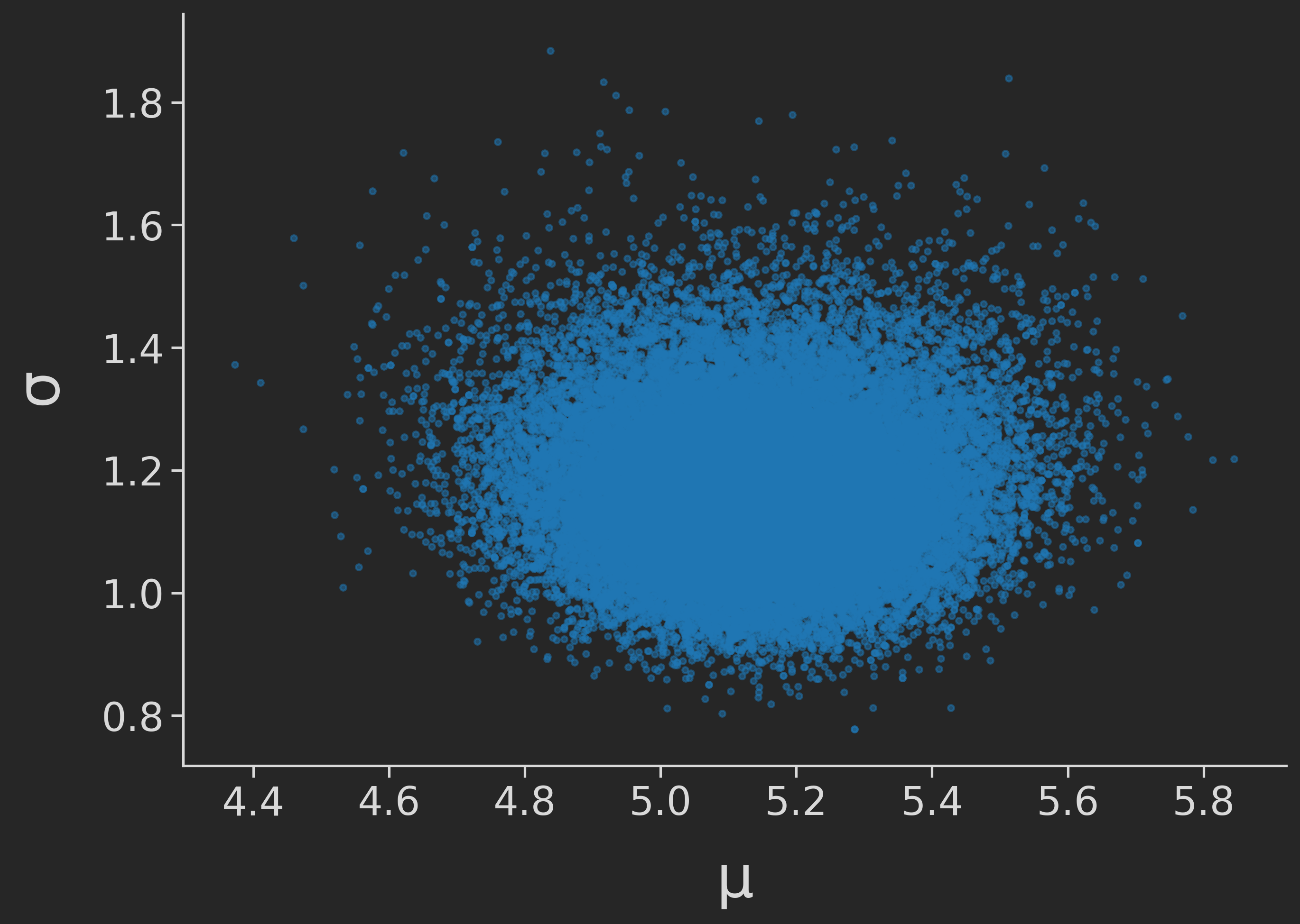
Looking good! Thus, we may proceed.

Predictive sampling

We might now be interested in quantifying the chance that a new data point in the future exceeds a certain value. Returning to our example, we might e.g. have found out that a concentration over 7 mg/ml of our marker elevates the risk of a certain disease, and we want to quantify the chance that a random patient falls into that group.

Since we have posterior distributions for the two parameters of our Gaussian distribution, we can quantify this probability by sampling values from a "distribution of distributions." This is what's called "predictive sampling." Using PyMC3, this is done as follows:

from pymc3 import sample_posterior_predictive

# Predictive sampling
with gauss_model:
    pp_samples = sample_posterior_predictive(samples, 1000)

# How many samples exceed our cutoff of 7?
print ((pp_samples['dist'] > 7).mean())

This gives us a probability of approximately 5.7% that a random patient in the future will exceeds the threshold of 7.0 mg/ml marker concentration.

Conclusion

In this post, we have learned the basics of Bayesian Inference, both from a theoretical/mathematical point of view, as well as from a practical point of view using the PyMC3 library for Python. Generally, we have fitted distributions to our raw data, and then answered questions about our datasets by examining the obtained posterior parameter distributions.In this way, we were able to assess the uncertainty of our parameter estimates and the likelihood of a random data point falling into a certain pre-specified range.

Of course, significantly more complex models can also be fitted using Bayesian inference. For the sake of brevity, we have not done so here, but we will come back to it in a future post which will we published here soon. In particular, we will e.g. deal with fitting a simple linear regression the Bayesian way. Stay tuned!