A small NLP data science project from start to finish
Posted: 21st November 2021Introduction
In this post, we will look at a little data science project I recently finished. I mostly did this for fun, but also for learning the basics of natural language processing (NLP), and to also try my hands at some web scraping.
Thematically, we will be dealing with the analysis of a small corpus of ~1000 letters exchanged between two famous German poets from the 18th and 19th century: J. W. v. Goethe and F. v. Schiller. Admittedly, the exact results are probably only interesting for a smaller group of people. Nonetheless, I think the general analytic approach and some general 'lessons learned' might be interesting for a wider audience. Also, I suspect that this post might even serve as a little tutorial or inspiration for people who are just starting out with the topic of web scraping and NLP.
Getting started
We will use the following Python libraries:requests, for downloading web pagesBeautifulSoup, for parsing web pagesscikit-learn, for text preprocessing and analysespandas, for working with data framenumpy, for statistics and general mathmatplotlib, for making plots
Apart from those, we will only need some standard Python libraries and a way to interact with jupyter notebooks.
All source code is available in the following github repository: Ma-Fi-94/Letters
Obtaining the raw data
(Check out the file scrape.py if you want to see the complete code for this section.)
Naturally, we first have to obtain our data. Here, this turned out to be pretty simple. The correspondence between Goethe and Schiller has been published as book multiple times already; and luckily, some of them are not copyrighted any more and can thus be freely found online. We will use the following set of thirteen chapters from the 1881 edition published by J. C. Cotta in Stuttgart, contained in two volumes, obtainable via Projekt Gutenberg here and here.
Using the `requests` library for Python, downloading the raw files becomes a matter of a few lines of code:
    r = requests.get('www.example.com')

    r.encoding = r.apparent_encoding

    with open('destinationfilename.html', 'w') as f:

        f.write(r.text)
Preprocessing the data
(Check out the file preprocess.py if you want to see the complete code for this section.)
Next, we need to preprocess the raw HTML files to extract the individual letters. The following section describes in detail what exactly I did. You may safely skip it, if you are not interested in that.
We loop over the downloaded HTML files, doing the following steps:
- Only extract the `body` of the HTML file, as all the information are in there. We use BeautifulSoup's
find("body")method for this. - Clean the contents of the
body: - Remove all footnotes, since those only contain annotations / additional information. In our case, this is done by removing all
<span>`s with BeautifulSoup'sdecompose(). - Remove all signatures. Luckily, in the HTML files there is a "signature" class for paragraph tags, so we just need to remove all
<p class="signature">`s, again using BeautifulSoup'sdecompose(). - For all remaining paragraphs, we remove the enclosing
<p>tags, using BeautifulSoup'sreplaceWithChildren(). - Remove all pictures and links, once again using BeautifulSoup's
decompose(). - Remove all enclosing boldface and italics tags, using BeautifulSoup's
replaceWithChildren(). - Find the positions of the letter beginnings in the current file. Luckily, they all start with a numbered heading, starting with the word "An", so we can use some simple regex magic to get them:
re.compile("[0-9]+\. An .+\.")does the trick. - Find the positions of the letter endings. In the HTML files, between every letter there is a
<hr>tag to generate a horizontal separating line between them. - Finally, extract the letters based on the positions extracted just before, and write them to a CSV file.
Data analysis – general principles
Now that we have stored all letters in a single CSV file, we can start working on the actual analyses. Such 'actual analyses' usually take the least amount of time in a project like this, compared to all the work to be done before. As the saying goes: Data science is mostly data obtaining, organising and cleaning.
To keep everything organised we will store our analyses in different jupyter notebook, splitted by the general type of question we want to answer. To avoid boilerplate code for e.g. importing the data, we will write some additional python scripts (with filenames lib_*.py), where we will store code we need multiple times. This allows allows for an easy testing of these external helper functions, which of course is a good thing in general to avoid errors.
First analysis: Letter counts and lengths by author and by time
(Check out the jupyter notebook Descriptive.ipynb if you want to see the complete code for this section.)
An excellent first step in any data analysis is simply looking at the data. Here, we will examine the numbers and lengths of the letters by author and over time. Such a simple inspection serves multiple purposes:
- First, it acts as a very easy sanity check -- if we only find three letters by one author, something clearly went wrong.
- Second, we gain a feel for and become more familiar with the dataset. This often gives rises to additional ideas and further questions to examine in the next steps.
- And finally, often at this very early stage of data analysis insights already pop up.
Let's start by simply counting how many letters our two authors have written by calling df.Author.value_counts(). We get:
| Author | Nb. Letters |
|---|---|
| Goethe |
521 |
| Schiller | 442 |
This appears realistic. However, the difference in numbers is interesting – is this a general trend? Let's examine cumulative letter counts over time. We count letters written by Goethe and by Schiller in two new columns, by adding a 1 to a cumulative count whenever a letter is written by the respective author:
    df["cum_counts_G"] = np.cumsum([1 if author == "Goethe" else 0 for author in df.Author])

    df["cum_counts_S"] = np.cumsum([1 if author == "Schiller" else 0 for author in df.Author])
Plotting these columns yields:

Interesting! There seems to be indeed a trend going on over the whole corpus with Goethe generally writing more often than his colleague.
Let's now look the average letter lengths. We calculate the length of every letter and then simply calculate the mean per author:
    df["length"] = [len(l) for l in df.Content]

    print(df.groupby("Author").mean().length)
We get (after some rounding):
| Author | Avg. Letter Length |
|---|---|
| Goethe |
1545 |
| Schiller | 2026 |
So on average, Schiller writes approximately 33% more than his collegue? No wonder he doesn't need to write that often ;-).
But wait, let's not get carried away too quickly and also inspect the raw data instead of only looking at summary statistics like the mean. After all, the mean is just a very rough summary of a dataset, easily affected by outliers, and not completely representative in case of skewed or bimodial distributions. We thus look at the raw distribution of letter lengths by author by simply generating a histogram.

Interesting again! While Goethe seems to mostly write short letters, his colleague shows a bimodal distribution. Schiller either writes rather short, or rather long letters. On average, this leads to a larger mean letter length; however, by looking only at summary statistics we never would have noticed.
Finally, let us also check again whether this trend persists over time. We calculate the cumulative sum of characters written by the two authors, as well as the cumulative sum of characters of all letters:
    df["cum_words"] = np.cumsum(df.length)

    df["cum_words_G"] = np.cumsum([length if author == "Goethe" else 0 for (length, author) in zip(df.length, df.Author)])

    df["cum_words_S"] = np.cumsum([length if author == "Schiller" else 0 for (length, author) in zip(df.length, df.Author)])
We get:

The difference between the two authors seems to persist over time. Interestingly, however, the writing speed (in characters per letter) of both writers seems to decline over time (an effect of old age, maybe ;-) ?). There are also some little spikes in the curves, hinting at short periods of higher productivity. Of course, since we only plot the index of the letters on the x-axis instead of the actual time, this might be confounded by differences in time passed between subsequent letters. A more thorough analysis could try to extract the data of every letter from the corpus to correct for that.
Second analysis: Which words change occurence over time?
(Check out the jupyter notebook Word_Frequencies_Over_Time.ipynb if you want to see the complete code for this section.)
Let's dig more deeply into the actual contents of the letters. A natural question we may want to answer is whether certain words change their frequency over time. Such words could represent topics that the authors care about more or less at different points of time. In contrast, words with a constant frequency over time are more likely to be non-informative 'everyday words' we don't really care about.
Let us first examine the distribution of word frequencies across the whole corpus:
| Nb. Occurences in Corpus | Number of Words | Fraction of Overall Nb. of Words |
|---|---|---|
| 1 | 9381 | 50.53% |
| 2 | 2788 | 15.02% |
| 3 | 1378 | 7.42 |
| 4 | 826 | 4.45 |
| 5 | 580 | 3.12 |
| 6 | 410 |
2.21 |
| 7 | 321 | 1.73 |
| 8 | 267 | 1.44 |
| 9 | 222 | 1.20 |
We notice that out of 18'567 different words, 9'381 words (which is more than 50%!) appear only once throughout the entire corpus. Additional 15%, 7.4%, 4.5%, and 3.1% of words appear only twice, thrice, four times, and five times, respectively. In other words, 80% of all words appear no more often than five times altogether. Rare words like these do not really lend themself to a direct analysis, so we want to apply some filtering: We remove all words, which do not appear at least fifty times across the complete corpus. This leaves us with 580 words – way easier to work with!
Now, we need to quantify the variability of occurences of a word across the letters. Calculating the standard deviation of counts is a good start, however since the standard deviation describes the 'absolut variability', it will be correlated with the average number of occurences. Hence, we calculate the coefficient of variation by dividing the standard deviation by the mean, to get the 'relative variabilities' of the words. In other words, we do:
C.V. = σ(x) / μ(x)
Words with a high coeeficient of variation (C.V.) are potentially interesting candidates to examine further.
Among the top twenty variable words, we find the following interesting candidates:
| Word | Sum Counts | Mean Counts | Stddev Counts | C.V. Counts |
|---|---|---|---|---|
| handlung | 52 | 0.053 | 0.385 | 7.141 |
| frankfurt | 51 | 0.062 | 0.373 | 7.051 |
| meister | 62 | 0.064 | 0.384 | 5.964 |
| faust | 55 | 0.057 | 0.331 | 5.805 |
| poesie | 62 | 0.064 | 0.370 | 5.750 |
| leser | 73 | 0.075 | 0.421 | 5.566 |
| almanachs | 52 | 0.053 | 0.293 | 5.443 |
| freiheit | 64 | 0.066 | 0.343 | 5.171 |
We notice some things which give rise to analyses presented in this post:
- "frankfurt" of course refers to the German town of the same name. It might be interesting to track the occurence of frankfurt over times, as well as some other cities as comparison.
- "meister", "faust", and "almanachs" refer to specific literary works, namely to Goethe's 'Faust', Goethe's 'Wilhelm Meisters Lehrjahre', and the "Musenalmanache" – collections of literary works compiled and edited by Schiller in the years 1796 to 1800. Thus, let's also track how often the titles of some of the works of the two authors appear in each letter.
Some other potential ideas, which we will not follow up on for the sake of brevity, could include:
- "poesie" (=poetry), "handlung" (=plot) and "leser" (=reader) refer to our two writers discussing the theory of their craft. In order to examine this more closely, one could track the frequency of words such as "poesie" (=poetry), "philosophie" (=philosophy), "kunst" (=art), etc.
- Finally, related to the first idea, it might also be cool to count how often the names of some famous contemporaries of Goethe and Schiller are mentioned. In other words, about whom do they share gossip and how often?
Towns
We start by looking at the word frequencies of certain towns. While plotting the count of a given word over time, one generally gets rather ugly curves. Because of the many zero values, the graph is dominated by flat horizontal lines and sharp peaks. Such a curve is hard to make sense of:

Hence, we will instead plot the _cumulative_ counts of a word over time:

Way better! Some insights immediately become apparent: The town of Weimar seems to be relevant throughout the whole corpus, whereas the town of Jena at some point starts to lose some of it relevance. This coincides perfectly with the point of time Schiller moved from Jena to Weimar (between 2nd and 4th of December 1799, letters 673 and 674, which have indices 638 and 639 in our dataset; but see the caveat later in this article). In contrast, the towns of Frankfurt and Berlin do not appear all too often in the letters and do not seem to be really relevant.
Books
Next, we look at how often certain books are mentioned.

There are a number of interesting things to see here.
- "almanach" clearly dominates the conversation. This makes sense, as the "Musenalmanache" were edited by Goethe and Schiller together, so it makes sense that they're a frequent topic of discussion. Also notice how the curve shows periods of faster vs. slower growth. The former correspond to those times, in which the books where in the final stage of preparation and were started to get distributed.
- "meister" (refering to Goethe's Wilhelm Meisters Lehrjahre) seems to be of intermediate interest for the two, and at some point their interest dies down, corresponding to the point of time in which the book was finished.
- "faust" is never really discussed until a certain point. This makes sense, since Goethe heavily procrastinated on completing his Faust, until Schiller at some point (around letter number 300-ish) convinced him to continue working on it.
- "dorothea" and "tasso" seem to be rather irrelevant in their discussion. Thus, apparently the two did not really talk much about Goethe's "Hermann und Dorothea" and his "Tasso" – which fits their rather minor role in the literary canon.
All in all, these trends nicely reflect what was happening in real life.
Third analysis: Do letters become more similar over time?
(Check out the jupyter notebook Letter_Similarities.ipynb if you want to see the complete code for this section.)
Finally, we move on to something slightly more involved. We want to answer the question whether the exchanged letters become more similar over time. To this end, we first need to transform the corpus into a structure that is easier to work with statistically. This can be achieved using a number of different approaches; here, we will use a rather simplistic one based on the Bag of Words model. In a bag of words model, for every document we count the raw occurences of all words of the corpus. We thus end up with a table with dimensionality n x m, where n represents the number of documents, and m the number of words of the corpus.
There are multiple different ways to construct this table:
- We can either simply track the raw counts of the individual words, or we could normalise these counts by the sum of counts of the respective word across all letters to avoid bias introduced by different baseline frequencies.
- We can also instead of tracking counts simply track the presence or absence of a word in a binary fashion.
- Additionally, we may want to specifiy a minimum length of words to consider to exclude short (and likely uninformative) words.
- Finally, instead of counting the occurence of words, we could also decide to track the occurence of 2-grams (or more generally: n-grams) instead – however given the rather small size of our corpus this is likely to not yield any insights.
We will experiment with the first three choices later in order to see how they might affect our results.
A typical bag of words table might thus look as follows:
| Word 1 | Word 2 | ... |
Word m | |
|---|---|---|---|---|
| Letter 1 | 0 | 1 | ... |
4 |
| Letter 2 | 1 | 0 | ... | 0 |
| ... | ... | ... | ... | ... |
| Letter n | 1 | 2 | ... | 0 |
In Python, such a table is easy to construct by using scikit-learn`s CountVectorizer, invoking:
    # Lengths of words we want to include

    minimum_word_length = 3

    maximum_word_length = 1000


    # Which n-grams to consider

    n_min = 1

    n_max = 1


    # Binary presencen/absence data, or counts?

    binary = False


    # Fit the model

    token_pattern = "\[a-zA-Z\]{" + str(mininum_word_length) + "," + str(maximum_word_length) +"}"

    model = CountVectorizer(ngram_range=(n_min, n_max), token_pattern=token_pattern, binary=binary)


    # Get results

    table = model.fit_transform(corpus)

    word_names = model.get_feature_names()
After having constructed our bag-of-words table, we need to come up with a metric to quantify the similarity of two documents, which here means quantifying the similarity between two rows of the table. Different distance or similarity metrics are available; here, we will use the Cosine similarity, which is often used for purposes like that.
Intuitively, the cosine similarity quantifies the divergence between two vectors in our m-dimensional space. More precisely, the cosine similarity S corresponds to the cosine of this angle θ, and can be calculated as follows:
S(A, B) := cos(θ) = A · B / (||A|| · ||B||)In Python, we can simply use the function sklearn.metrics.pairwise.cosine_similarity(X), where X contains the vectors to compare.
Note that other, more familiar metrics such as the Euclidean distance, are likely not a good choice because these tend to fail in higher dimensions. As Pedro Domingos has put it in this paper:
[O]ur intuitions, which come from a three-dimensional world, often do not apply in high-dimensional ones. In high dimensions, most of the mass of a multivariate Gaussian distribution is not near the mean, but in an increasingly distant “shell” around it; and most of the volume of a high-dimensional orange is in the skin, not the pulp. If a constant number of examples is distributed uniformly in a high-dimensional hypercube, beyond some dimensionality most examples are closer to a face of the hypercube than to their nearest neighbor. And if we approximate a hypersphere by inscribing it in a hypercube, in high dimensions almost all the volume of the hypercube is outside the hypersphere.
Fitting the bag of words model and computing all pair-wise cosine similarities (for 1-grams with minimum word length of 3 characters, unnormalised and non-binarised counts) between the letters gives us the following similarity matrix:
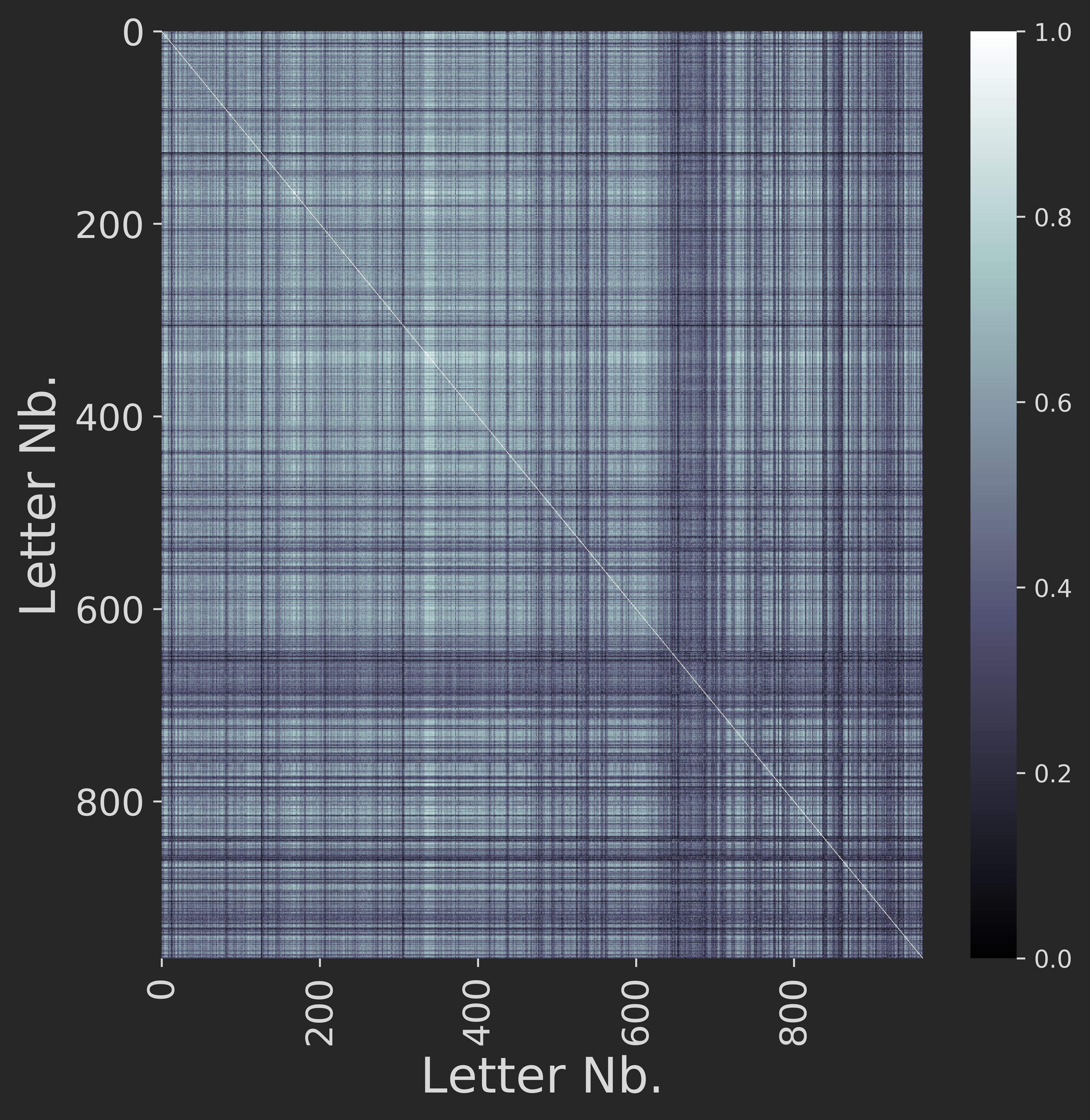
We now slide a window of length 100 over the sequence of letters and compute the average pair-wise letter similarity over time. We get:
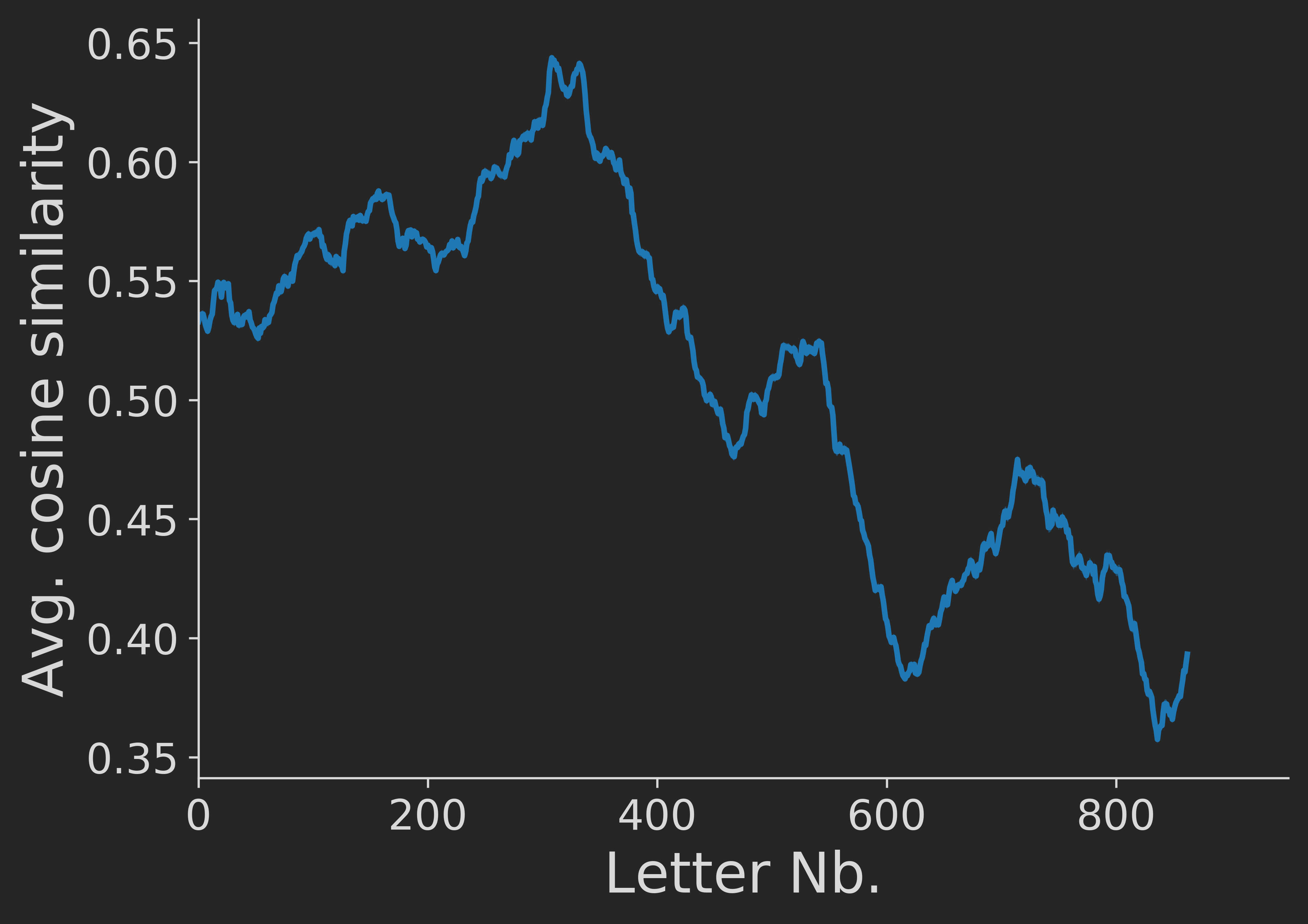
Interesting – apparently, the pair-wise letter similarity on average actually decreased over time. In order to check the robustness of this finding, we re-run the analysis with different window sizes, getting similar results:
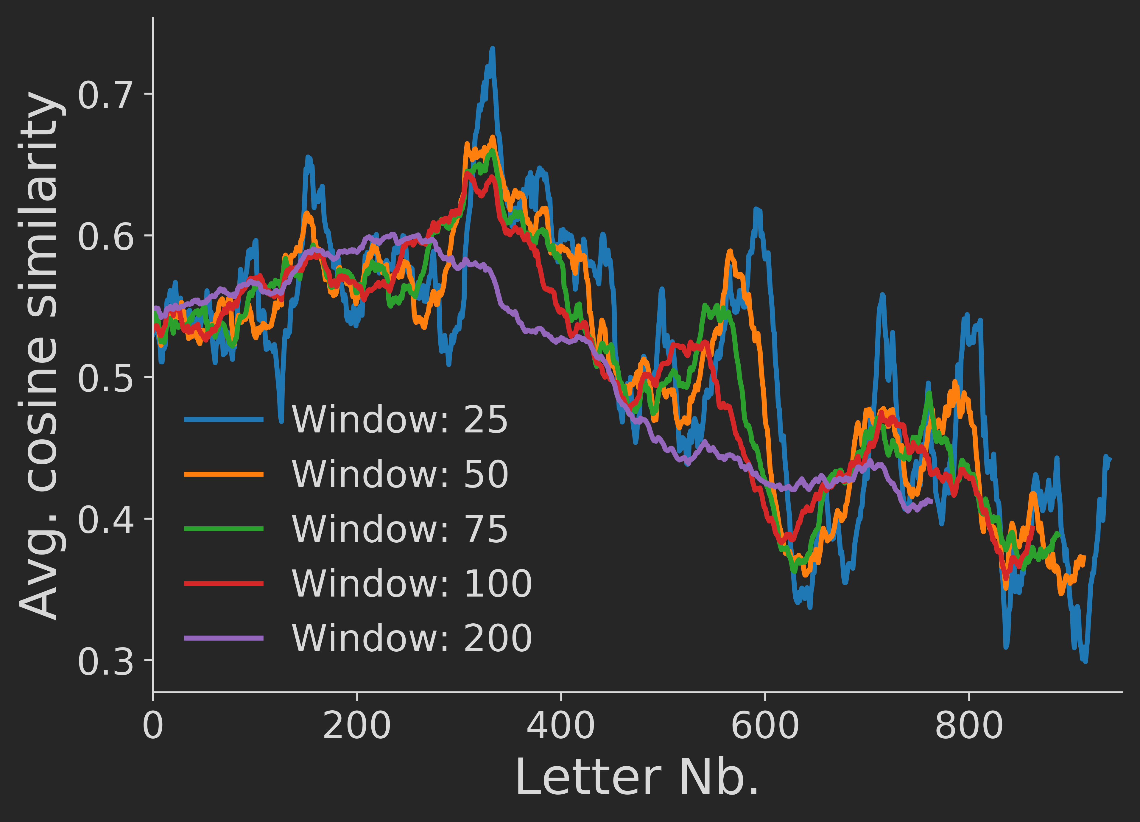
Thus, apparently over time the two writers did not "find a common style", but instead seemed to actually have separated stylistically.
We now want to check how robust this result is to changes in the analytic approach. If we change the minimum letter length to 1, 5, or 10, instead of 3 letters, we get extremely similar results (not shown here for brevity, can be reproduced from the jupyter notebook). The result also stays the same if we switch to binary presence/absence data instead of using the raw word counts (again not shown here). However, a completely different result emerges when we normalise word counts across letters:
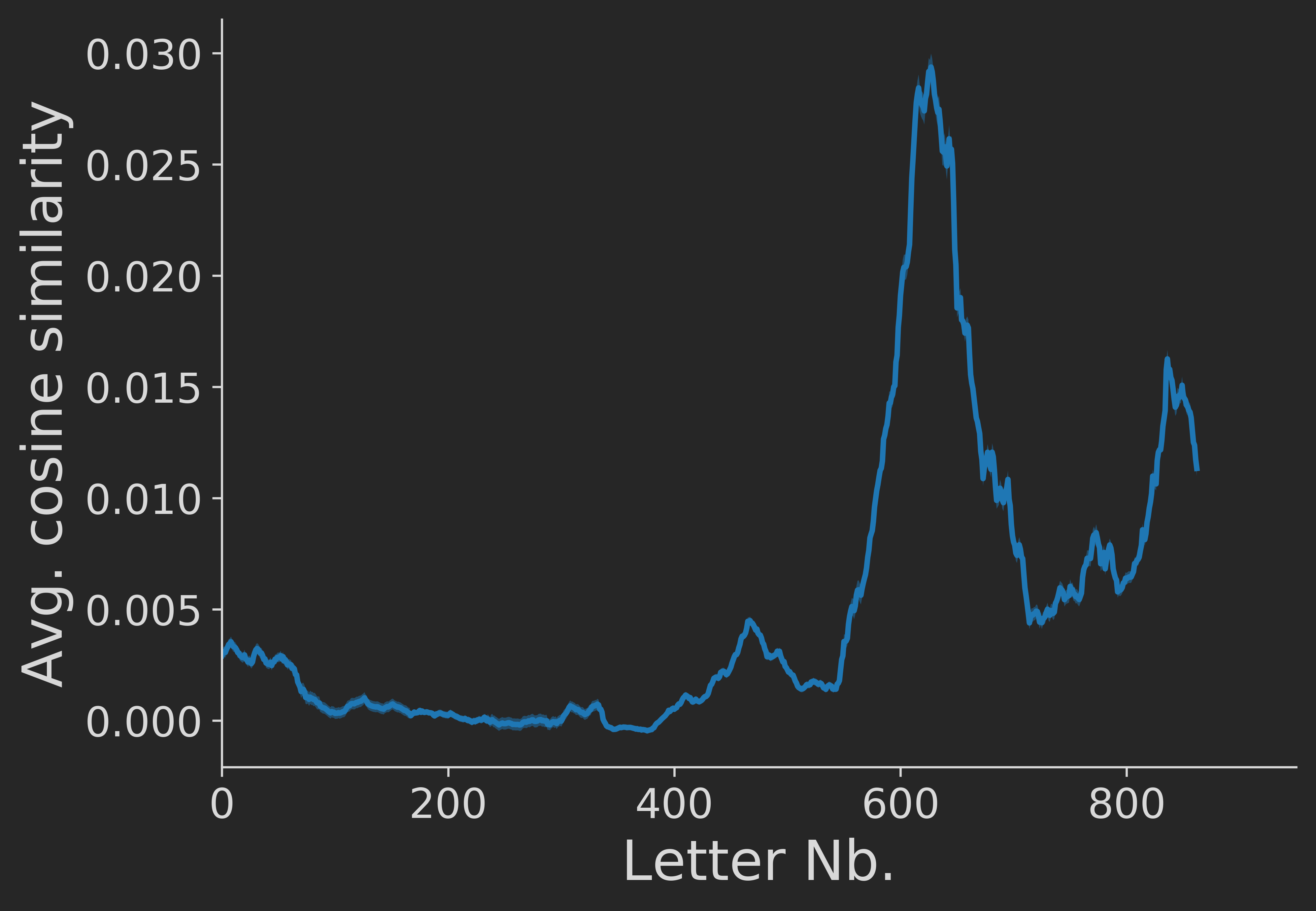
Using normalised word counts, we get the impression that around letter 600-ish there is a huge spike in avergae letter similiarity, after which a second spike emerges. Thus, qualitatively completely different results can emerge if we change the analytic approach. To judge which is the "right" approach requires a more precise definition of our question:
When we normalise the counts of a word across letters we limit the (formally rather big) relative influence of the mroe frequent words on the vectors, whereas rarer words will now influence the vectors more strongly. Thus, in the normalised scenario, all words contribute equally to the letter vectors, regardless of whether they're used frequently or infrequently throughout the corpus. In contrast, in the non-normalised scenario more frequent words exert a bigger influence on the data. For answering the question whether the two authors over time deelop a "common style" of talking, I think the non-normalised approach is more appropriate.
Conclusions, caveats and a little outlook
This was a very fun 'end to end' project that has taught me quite a lot! From writing a simple scraper for getting raw data, over dealing with the nitty-gritty details of data cleaning and preprocessing, to developing questions to ask, all the way to actually performing these analyses and interpreting their results – this project has consisted of all the major steps one needs to perform in a 'real-world' project too.
Some ideas (in no particular order) for future tinkering:
- Trying to extract the date from the letters. Usually it's placed right at the top in square brackets, or somewhere in the last paragraph of a letters. Using some regex magic, this should actually be doable rather easily, I think. Then, one could examine temporal trends in letter writings, average time between letters by the two author, whether times between letters and their lengths are correlated, etc.etc.
- In a similar vein: extract the town names written next to the date in (nearly) every letter. In the analysis earlier, we have counted the town names as parts of the letter texts which is probably the reason why Weimar and Jena show up that often. It would be interesting to see how often the two authors talk about these towns if we exclude those occurences.
- Examining co-occurences of words. Are there pairs of words that tend to appear together more often than one would expect from pure chance alone?
- Sentiment analysis. This is a bit tricky, because the letters are written in German, and the writing style is noticeably old -- so quantifying sentiment from these texts is not that straightforward, I suspect.
Some take-home messages:
- Data loading, cleaning, and organising are the first, and generally most time-consuming steps in data science.
- They are also the most important steps for getting useful and reliable results. See also: Garbage In, Garbage Out
- Inspect the data, before doing any elaborate analyses. This is standard advice in many statistics textbooks – and rightfully so. This way, you get to know your data, can spot obvious mistakes, and get inspiration for further questions to examine. Check out Anscombe's Quartet to see the importance of visually inspecting your data.
- The results of more elaborate analyses can strongly depend on the settings and parameters used. This is where domain knowledge, a precise definition of our research question, and an in-depth understanding of our analytic methodology can help to guide analyses.